Introduction to Accelerometer Data
Common Data Formats
- Raw Accelerometer Data (high-resolution time-series data)
- Activity Counts (aggregated over time windows)
- Wear Time Detection (non-wear vs. wear periods)
- Steps (estimation of a “step”)

Time (data) is not your friend
- Time zones are hell
read.gt3xattached a GMT timezone to the data, but there is a note
- “local” means local to the device/initialization, not your machine
Can do tz<- to change the timezone if you want (watch out for DST):
Plot First 5 minutes (30Hz dense)
library(ggplot2); library(lubridate)
(qp = long %>%
    filter(between(time, floor_date(time[1]),
                   floor_date(time[1]) + as.period(5, "minutes"))) %>%
    ggplot(aes(x = time, y = acceleration, colour = axis)) +
    geom_rect(aes(xmin = ymd_hms("2017-10-30 15:00:22"),
                  xmax = ymd_hms("2017-10-30 15:00:37"),
                  ymin = -Inf, ymax = Inf), fill = 'pink', alpha = 0.05) +
    geom_line())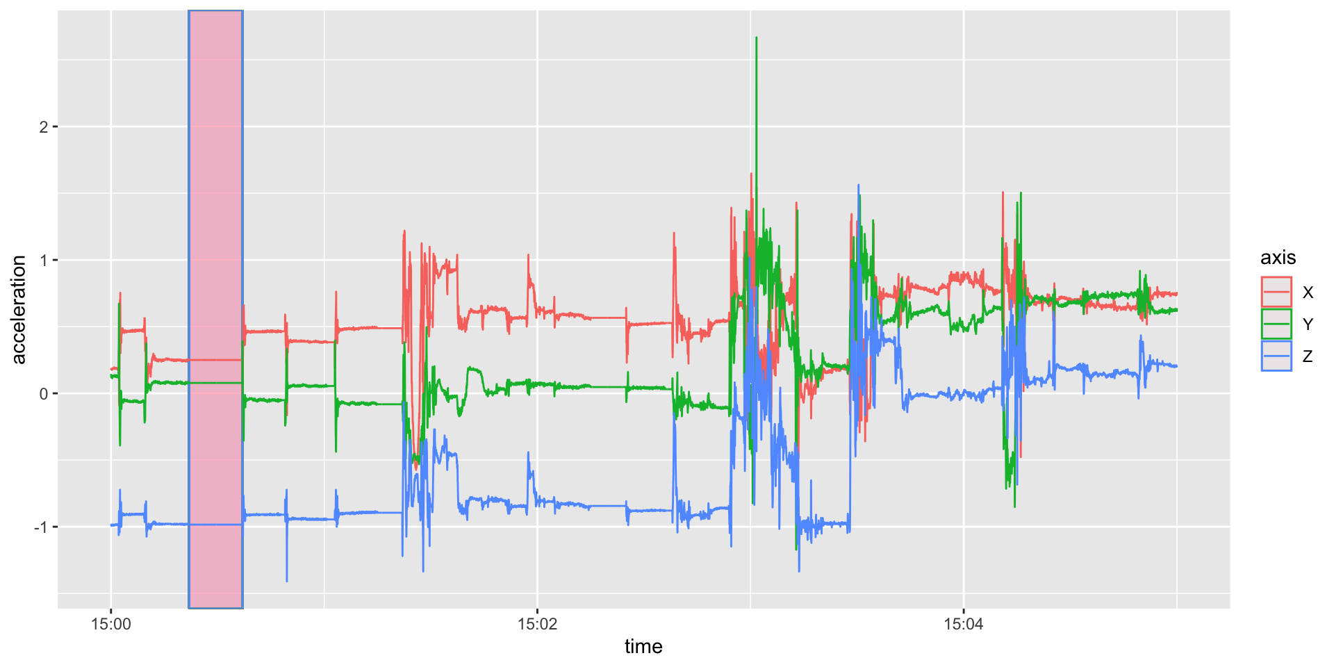
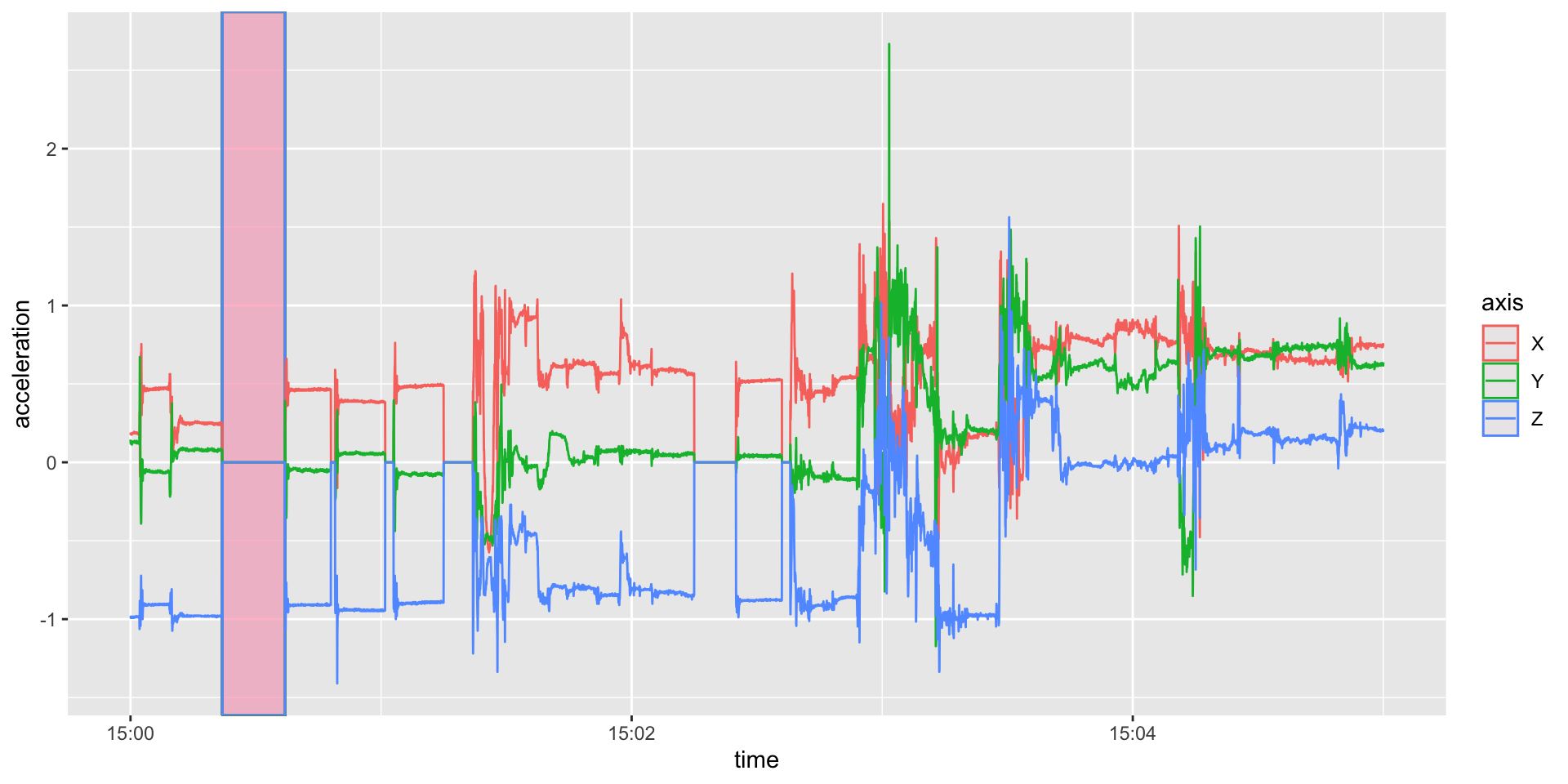
Same Plot with Zeroes
Plot all data
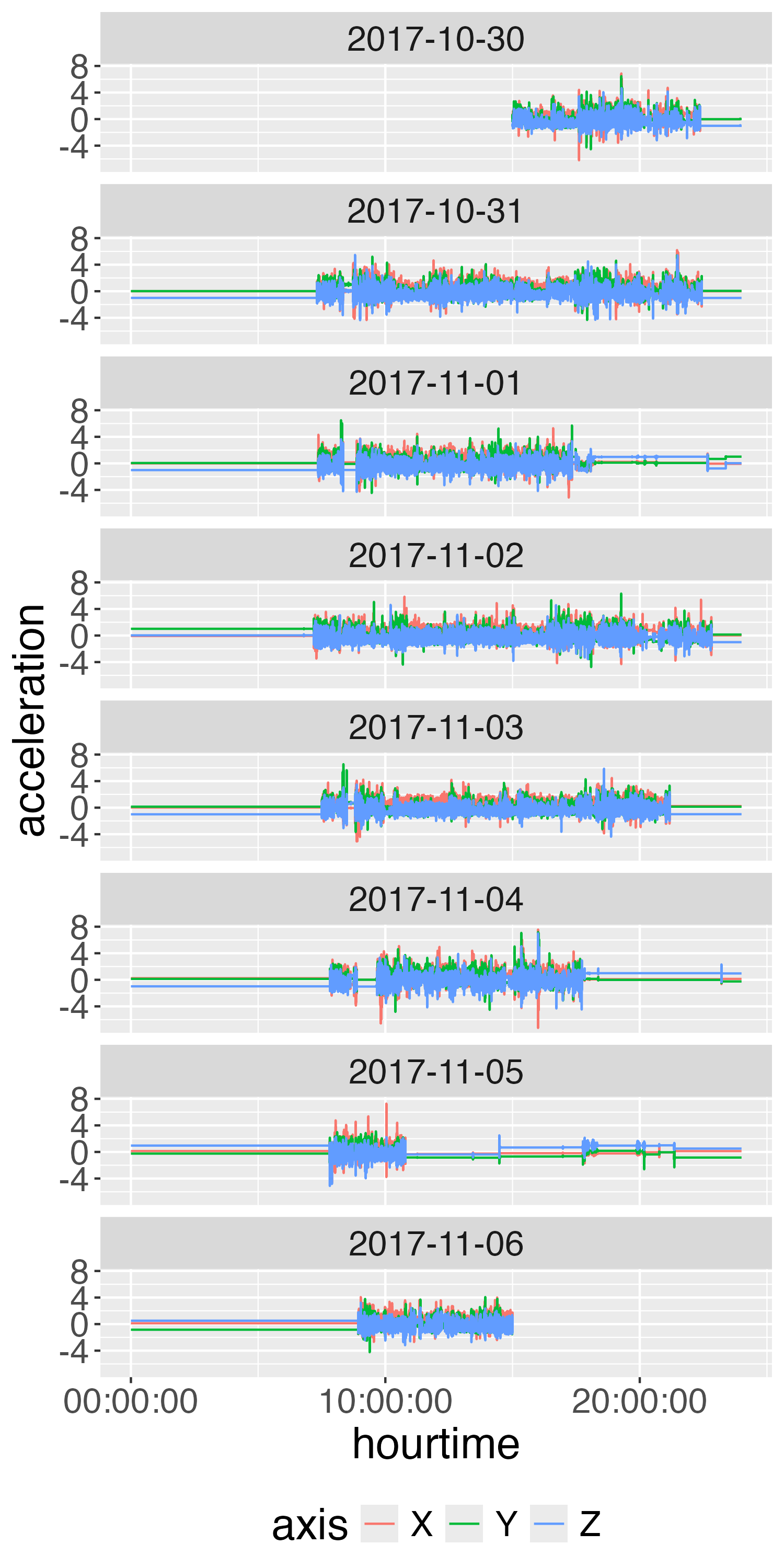
Plot Second-Level Data
Take average over each axis and plot
long %>%
  mutate(time = floor_date(time, unit = "1 second")) %>%
  group_by(time, axis) %>%
  summarise(
    acceleration = mean(acceleration, na.rm = TRUE), .groups = "drop"
  ) %>%
  mutate(date = as_date(time),
         hourtime = hms::as_hms(time)) %>%
  ggplot(aes(x = hourtime,
             y = acceleration,
             colour = axis)) +
  facet_wrap(~ date, ncol = 2) +
  geom_step() +
  theme(text = element_text(size = 15)) +
  guides(colour = guide_legend(position = "bottom"))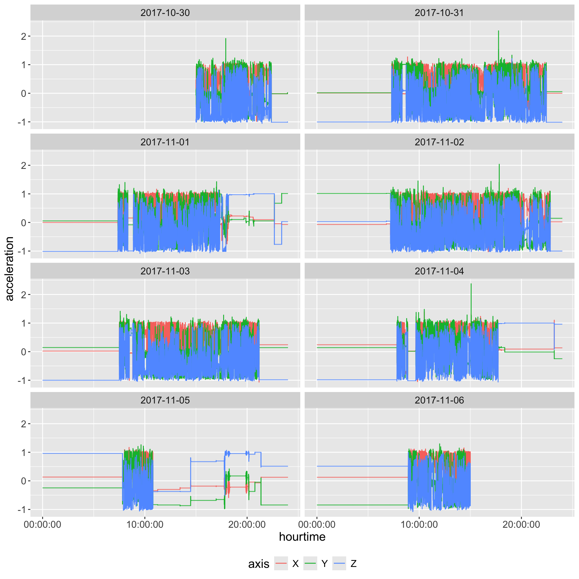
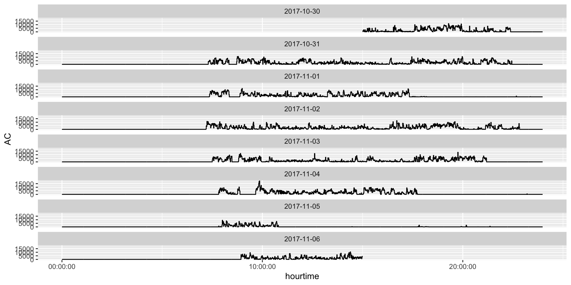
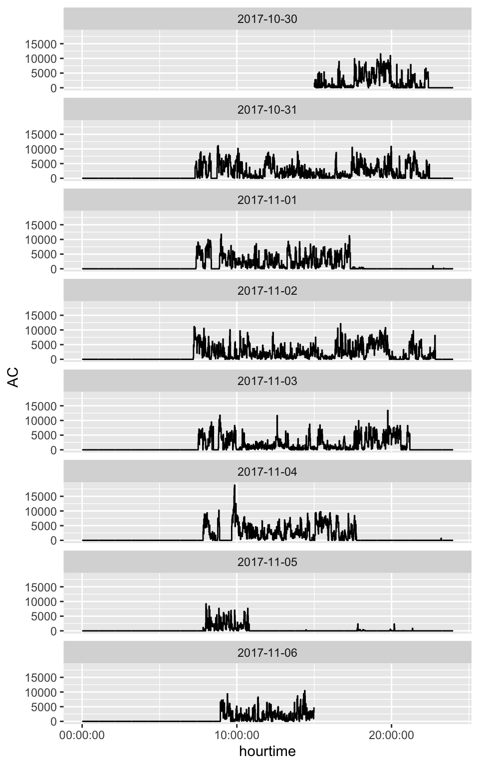
Plotting Activity Counts
Plotting Non-wear
Overall, this looks like relatively clean data, but there are some segments (e.g. 2017-11-01 at 20:00) that may be misclassified.
data %>%
  rename(time = timestamp) %>%
  mutate(date = lubridate::as_date(time),
         hourtime = hms::as_hms(time)) %>%
  ggplot(aes(x = hourtime, y = AC)) +
  geom_segment(
    aes(x = hourtime, xend = hourtime,
        y = -Inf, yend = Inf, color = choi_wear), alpha = 0.25) +
  geom_line() +
  guides(color = guide_legend(position = "top")) +
  facet_wrap(~ date, ncol = 1)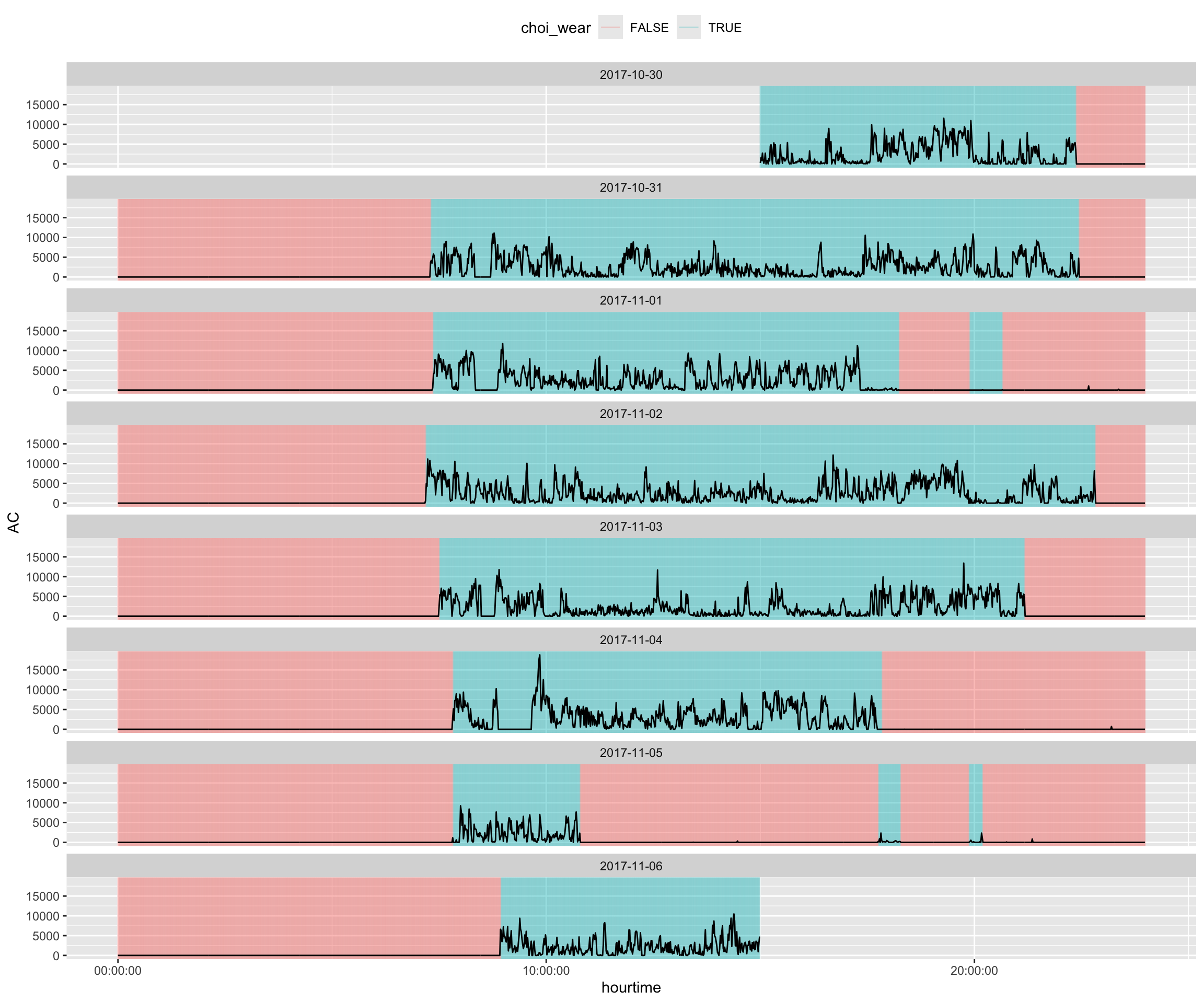
MIMS Units
MIMSunit package - calculate Monitor-Independent Movement Summary unit (John et al. 2019):
- interpolation of the signal to 100Hz,
- extrapolate signal for regions that have hit the maximum/minimum acceleration units for the device
- band-pass filter from 0.2 to 5Hz,
- absolute value of the area under the curve (AUC) using a trapezoidal rule,
- truncates low signal values to \(0\).
You may need to rename the time column to HEADER_TIME_STAMP for MIMS units depending on the version of the package:
    HEADER_TIME_STAMP MIMS_UNIT
1 2017-10-30 15:00:00  7.586073
2 2017-10-30 15:01:00 12.369848
3 2017-10-30 15:02:00  9.468913
4 2017-10-30 15:03:00 15.628471
5 2017-10-30 15:04:00  7.354169
6 2017-10-30 15:05:00  7.216364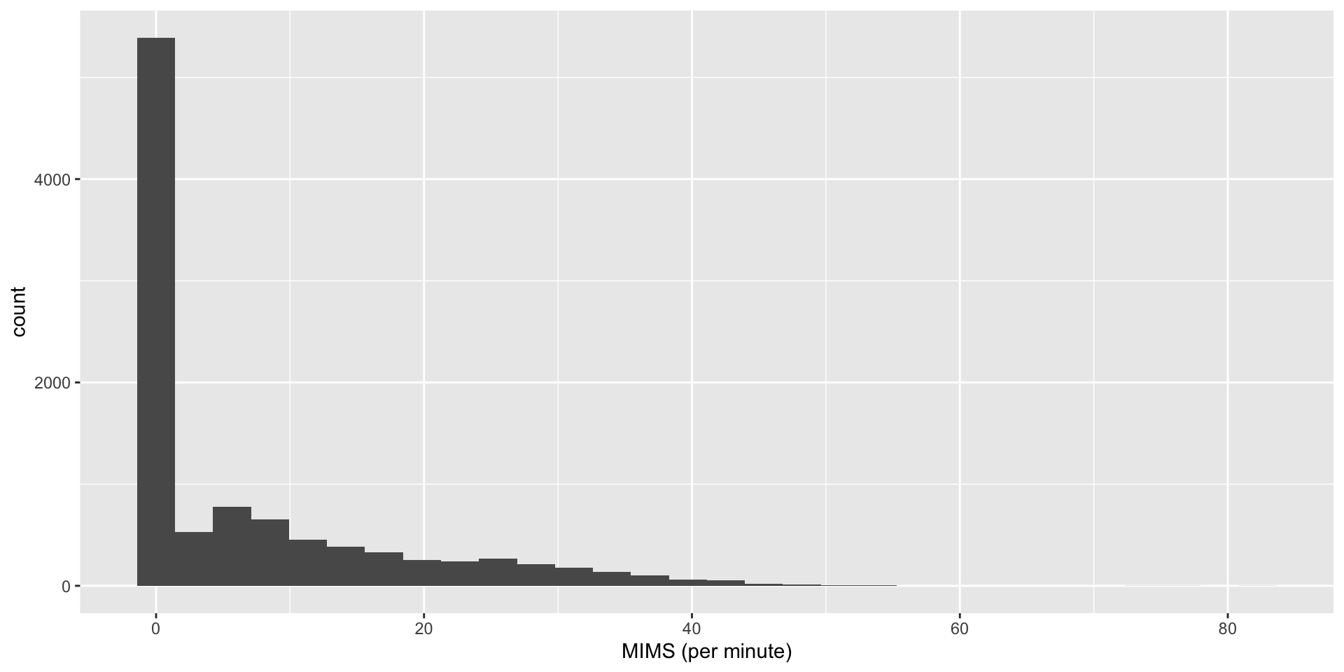
Compare MIMS and AC
Karas et al. (2022) found a correlation of \(\geq 0.97\) between AC and MIMS units.
joined = ac60 %>%
  full_join(mims %>%
              rename(time = HEADER_TIME_STAMP))
cor(joined$AC, joined$MIMS_UNIT)
[1] 0.9844991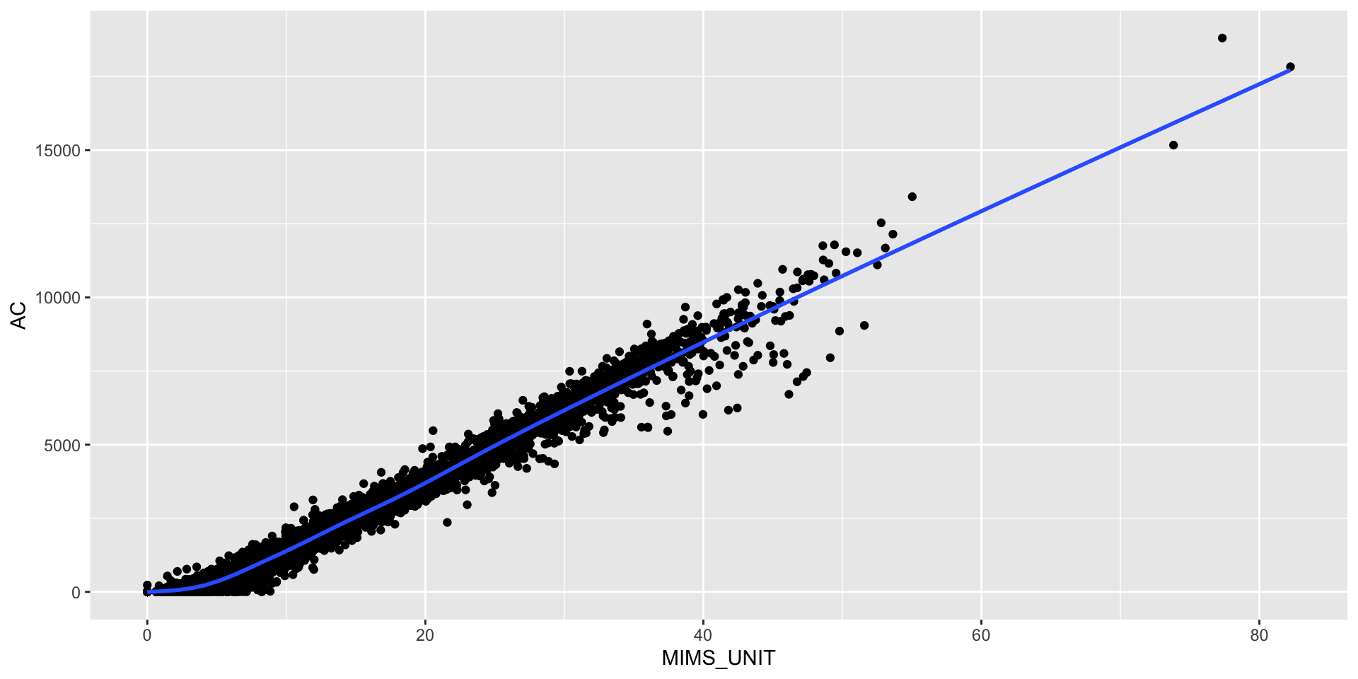
Step Counts
The output of stepcount is a list of different pieces of information, including information about the device:
A data.frame of flags for walking:
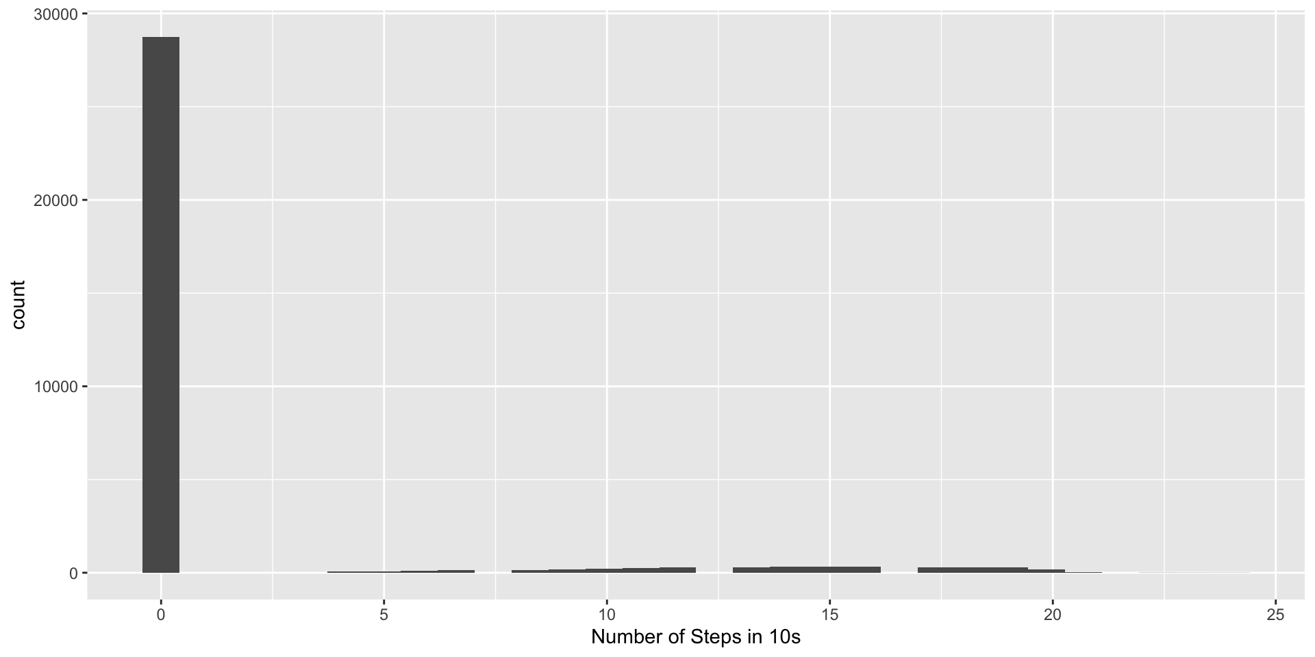
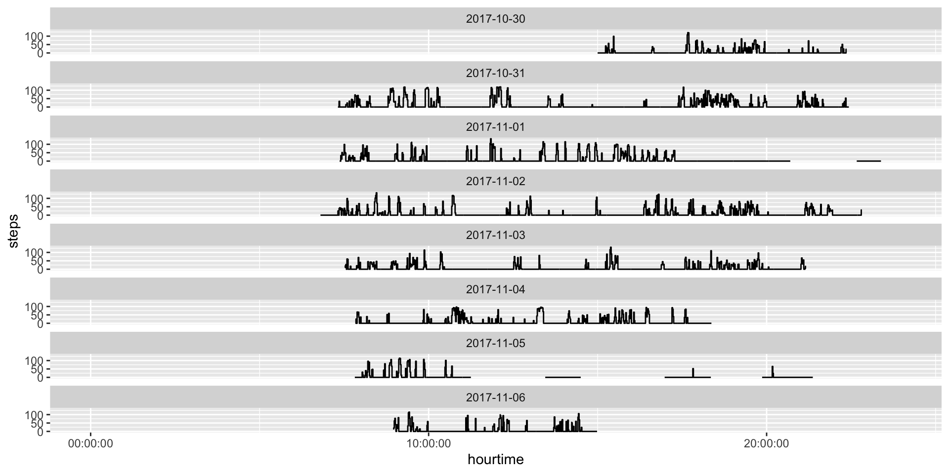
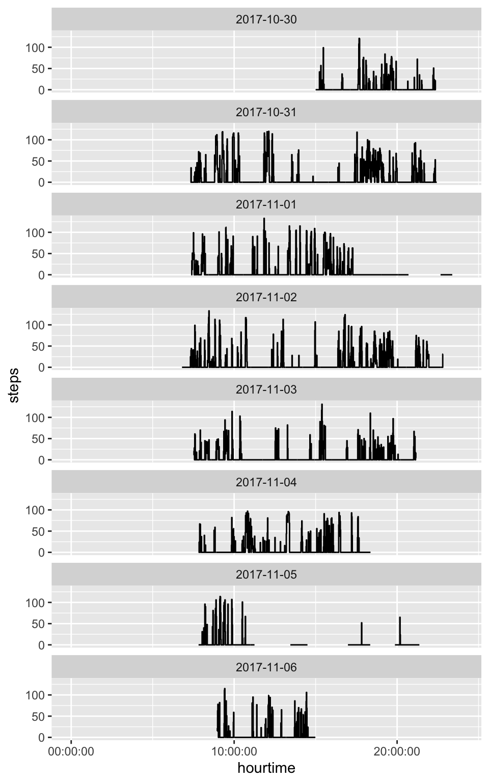
Steps Per Minute
Steps vs AC
References

Chadwell, Alix, Laurence Kenney, Malcolm Granat, Sibylle Thies, Adam Galpin, and John Head. 2019b. “Upper Limb Activity of Twenty Myoelectric Prosthesis Users and Twenty Healthy Anatomically Intact Adults.” Scientific Data 6 (1): 199.
Choi, Leena, Zhouwen Loiu, Charles E. Matthews, and Maciej S. Buchowskie. 2011. “Validation of Accelerometer Wear and Nonwear Time Classification Algorithm.” Medicine & Science in Sports & Exercise 43 (2): 357–64. https://doi.org/10.1249/mss.0b013e3181ed61a3.
Hees, Vincent T. van, Zhou Fang, Joss Langford, Felix Assah, Anwar Mohammad, Inacio C. M. da Silva, Michael I. Trenell, Tom White, Nicholas J. Wareham, and Søren Brage. 2014. “Autocalibration of Accelerometer Data for Free-Living Physical Activity Assessment Using Local Gravity and Temperature: An Evaluation on Four Continents.” Journal of Applied Physiology 117 (7): 738–44. https://doi.org/10.1152/japplphysiol.00421.2014.
John, Dinesh, Qu Tang, Fahd Albinali, and Stephen Intille. 2019. “An Open-Source Monitor-Independent Movement Summary for Accelerometer Data Processing.” Journal for the Measurement of Physical Behaviour 2 (4): 268–81. https://doi.org/10.1123/jmpb.2018-0068.
Karas, Marta, John Muschelli, Andrew Leroux, Jacek K Urbanek, Amal A Wanigatunga, Jiawei Bai, Ciprian M Crainiceanu, and Jennifer A Schrack. 2022. “Comparison of Accelerometry-Based Measures of Physical Activity: Retrospective Observational Data Analysis Study.” JMIR mHealth and uHealth 10 (7): e38077.
Knaier, Raphael, Christoph Höchsmann, Denis Infanger, Timo Hinrichs, and Arno Schmidt-Trucksäss. 2019. “Validation of Automatic Wear-Time Detection Algorithms in a Free-Living Setting of Wrist-Worn and Hip-Worn ActiGraph GT3X+.” BMC Public Health 19: 1–6.
Neishabouri, Ali, Joe Nguyen, John Samuelsson, Tyler Guthrie, Matt Biggs, Jeremy Wyatt, Doug Cross, et al. 2022. “Quantification of Acceleration as Activity Counts in ActiGraph Wearable.” Scientific Reports 12 (1): 11958.
Small, Scott R, Shing Chan, Rosemary Walmsley, Lennart von Fritsch, Aidan Acquah, Gert Mertes, Benjamin G Feakins, et al. 2024. “Self-Supervised Machine Learning to Characterize Step Counts from Wrist-Worn Accelerometers in the UK Biobank.” Medicine and Science in Sports and Exercise 56 (10): 1945.
Troiano, Richard P, James J McClain, Robert J Brychta, and Kong Y Chen. 2014. “Evolution of Accelerometer Methods for Physical Activity Research.” British Journal of Sports Medicine 48 (13): 1019–23.