Plotting Minute-Level Activity Data

library(actiplot)

This vignette uses the packaged acti_minute_data accelerometer recording. It contains seven days of minute-level vector-magnitude activity counts. It is processed from the upper-limb activity Figshare collection described by Chadwell et al. (2019).

activity <- acti_minute_data

Complete recording

Use acti_plot_time() to inspect activity across the entire recording. The breaks argument accepts ordinary duration strings and sets the interval of the time-axis labels.

acti_plot_time(activity, counts, breaks = "4 hours")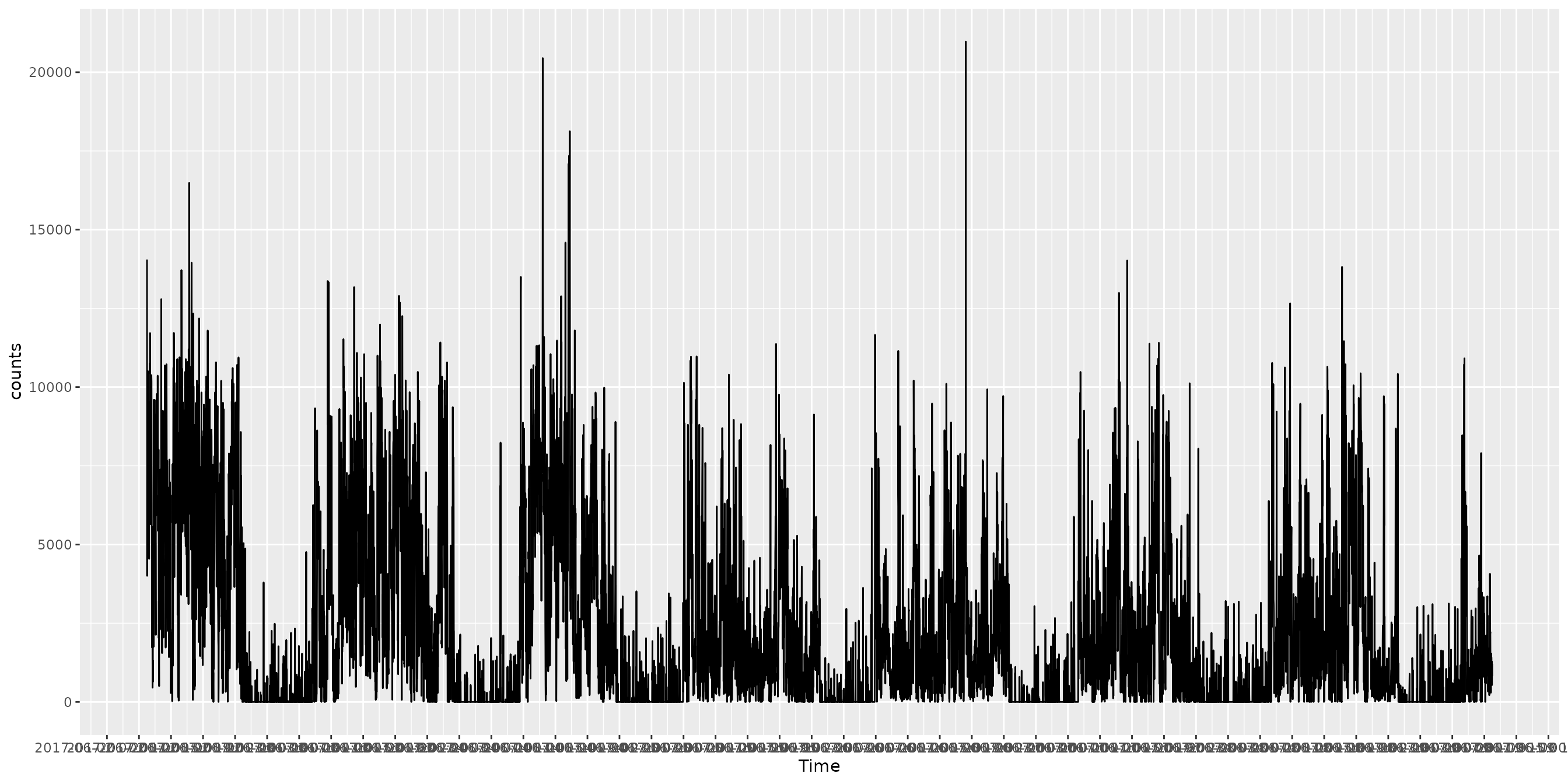

For a more legible complete-recording axis, set x_axis = "12 hours". It shows date and 12-hour-clock labels at midnight and noon. Alternatively, x_axis = "midnight" prints just the date at midnight, without 00:00:00.

acti_plot_time(activity, counts, x_axis = "12 hours")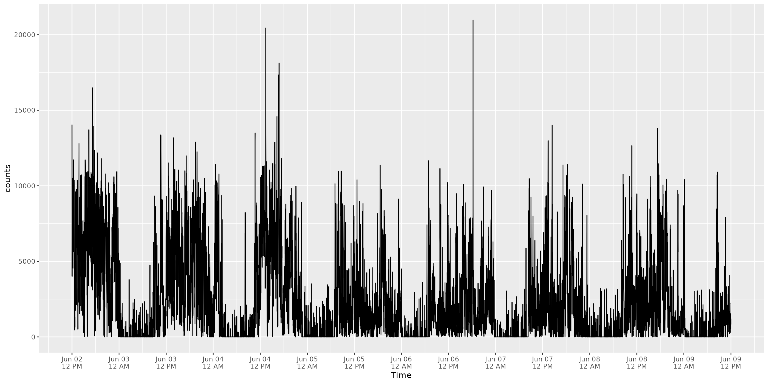

acti_plot_time(activity, counts, x_axis = "midnight")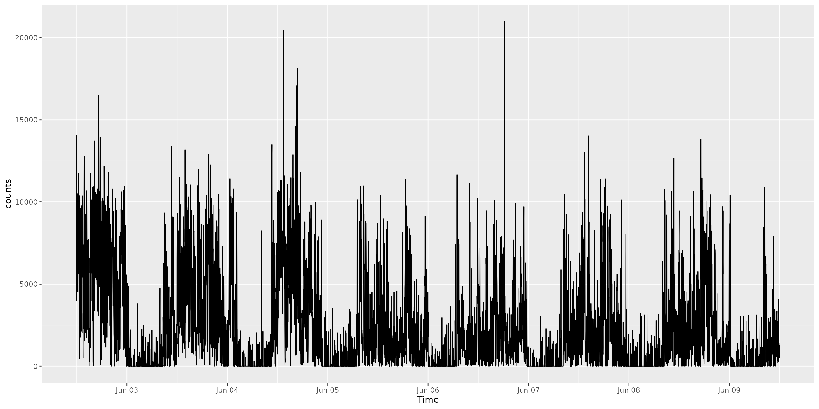

Daily aligned rows

Use acti_plot_day() to align each day on the same time-of-day axis. Each facet row is one calendar date, which makes day-to-day activity patterns easy to compare.

acti_plot_day(activity, counts, breaks = "4 hours")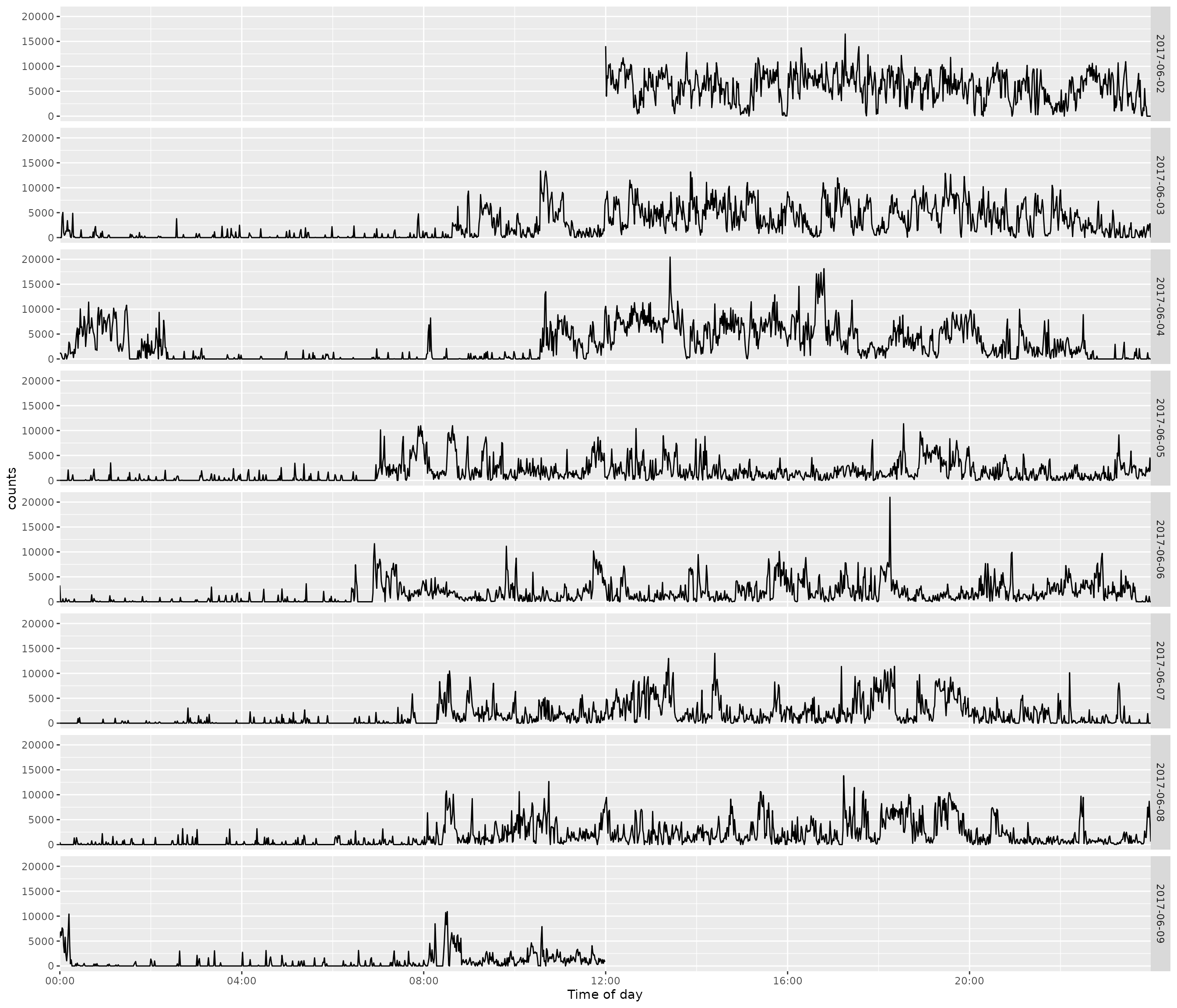

Set facet = "month-day" to remove the year from date strips, or facet = "day" to use the baseline-relative day calculated by actibase::acti_separate_times().

acti_plot_day(activity, counts, facet = "month-day")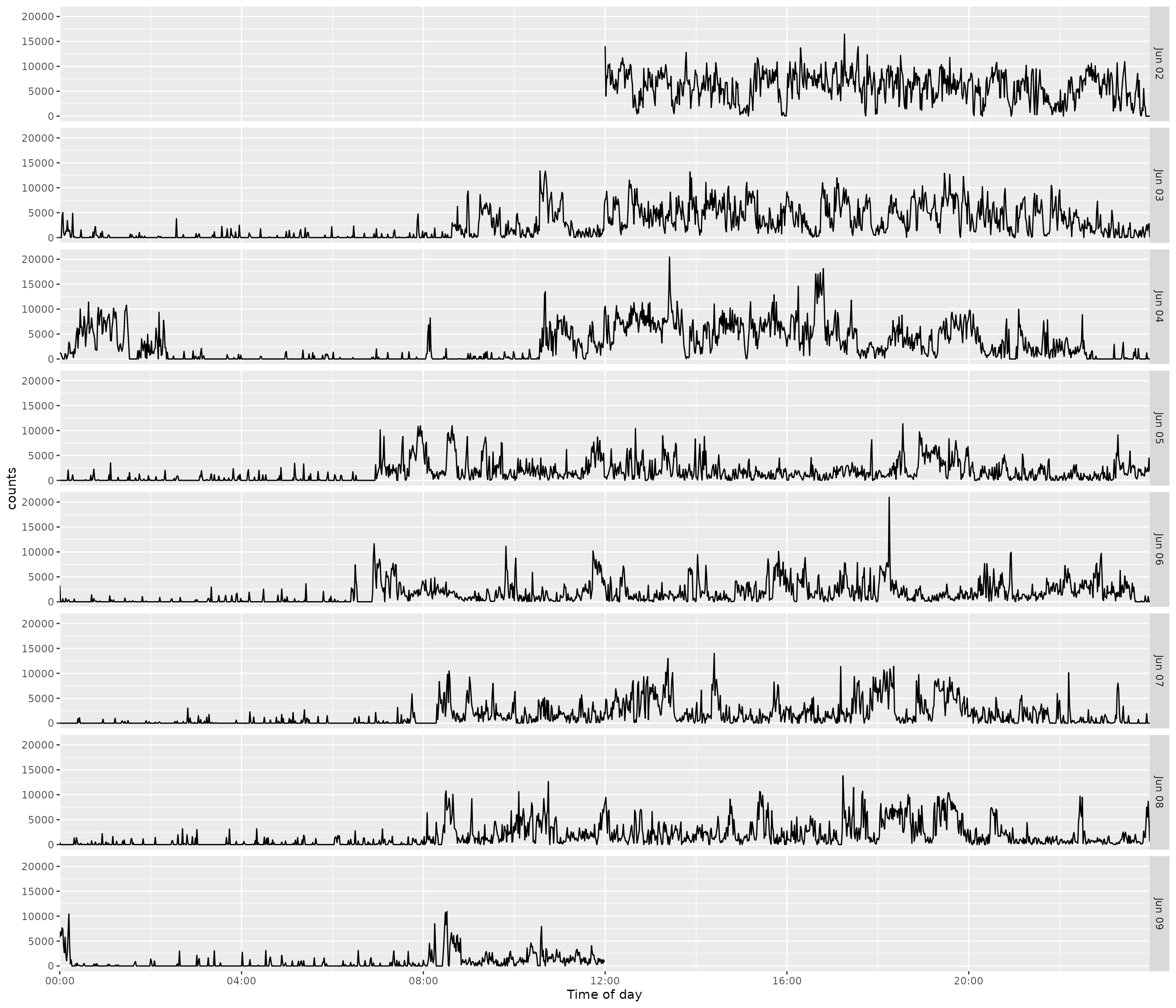

acti_plot_day(activity, counts, facet = "day")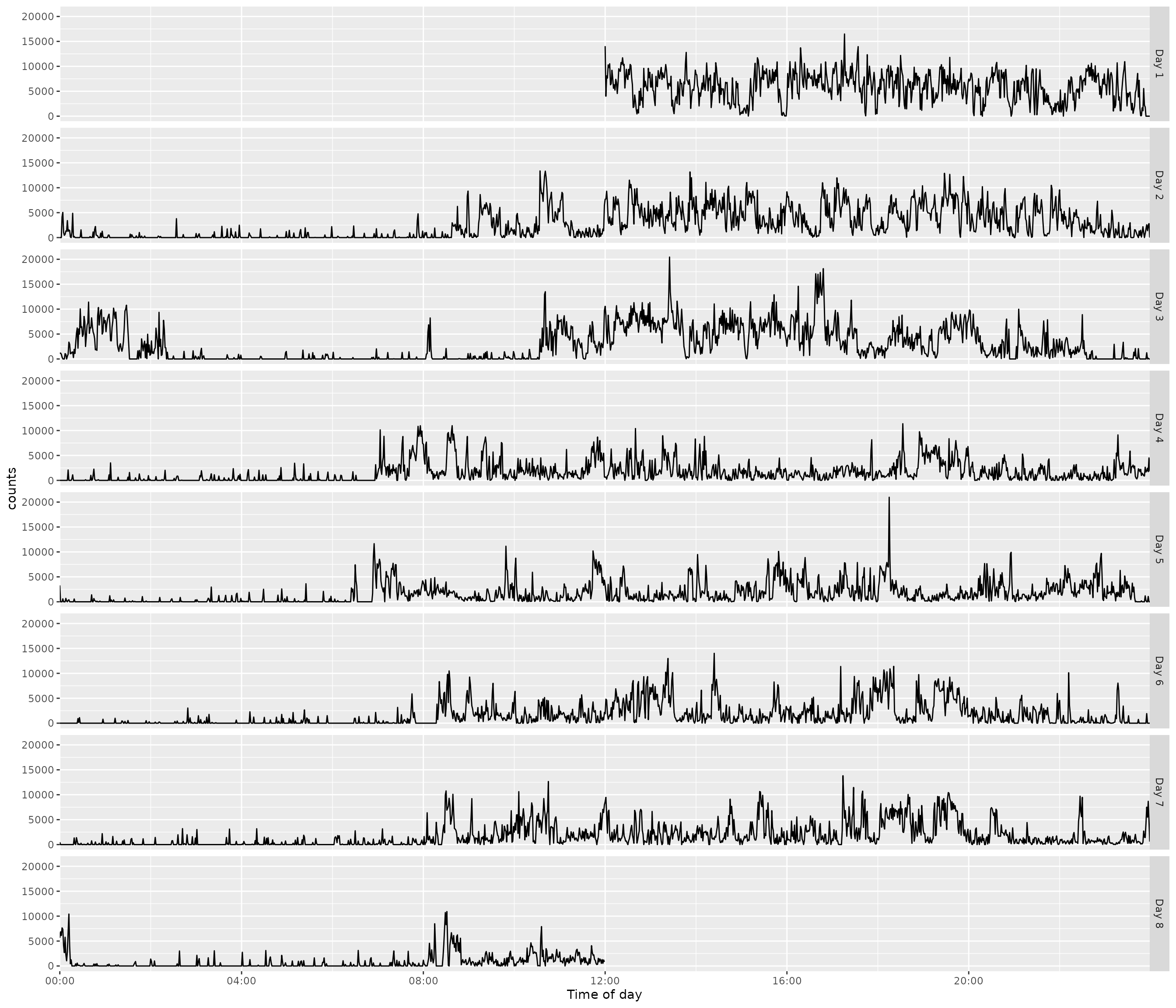

Date-by-time heat map

acti_plot_heatmap() uses the same alignment with counts represented by fill.

acti_plot_heatmap(activity, counts, breaks = "4 hours")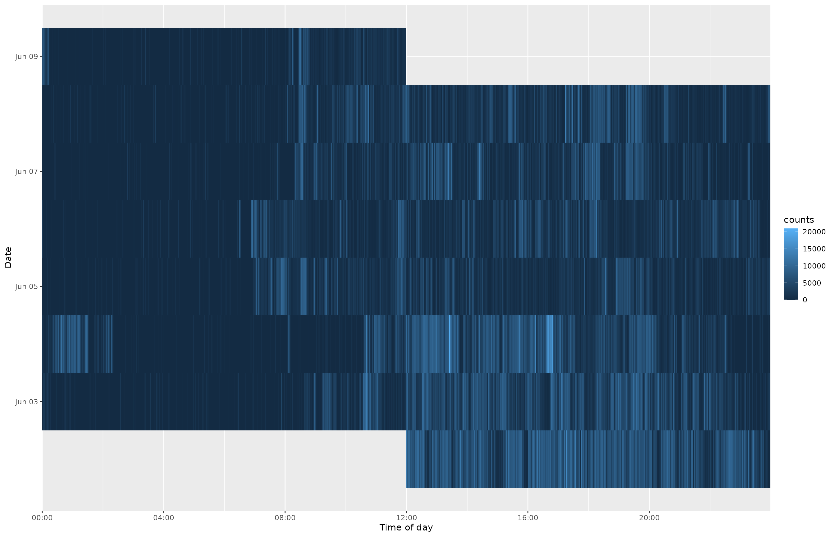

Actogram and daily profile

acti_plot_actogram(activity, counts, breaks = "4 hours")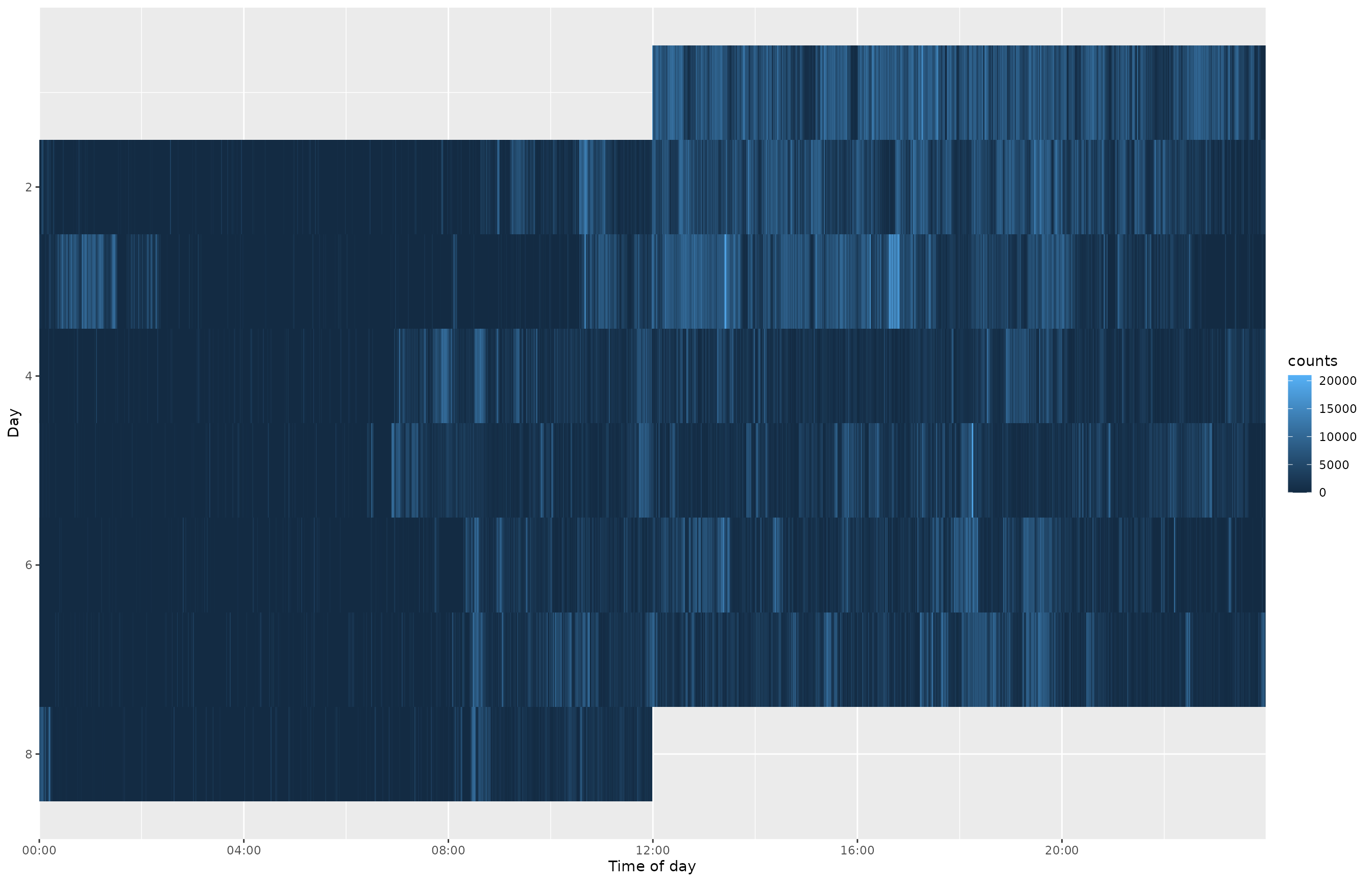

acti_plot_minute_profile(activity, counts, summary = "median")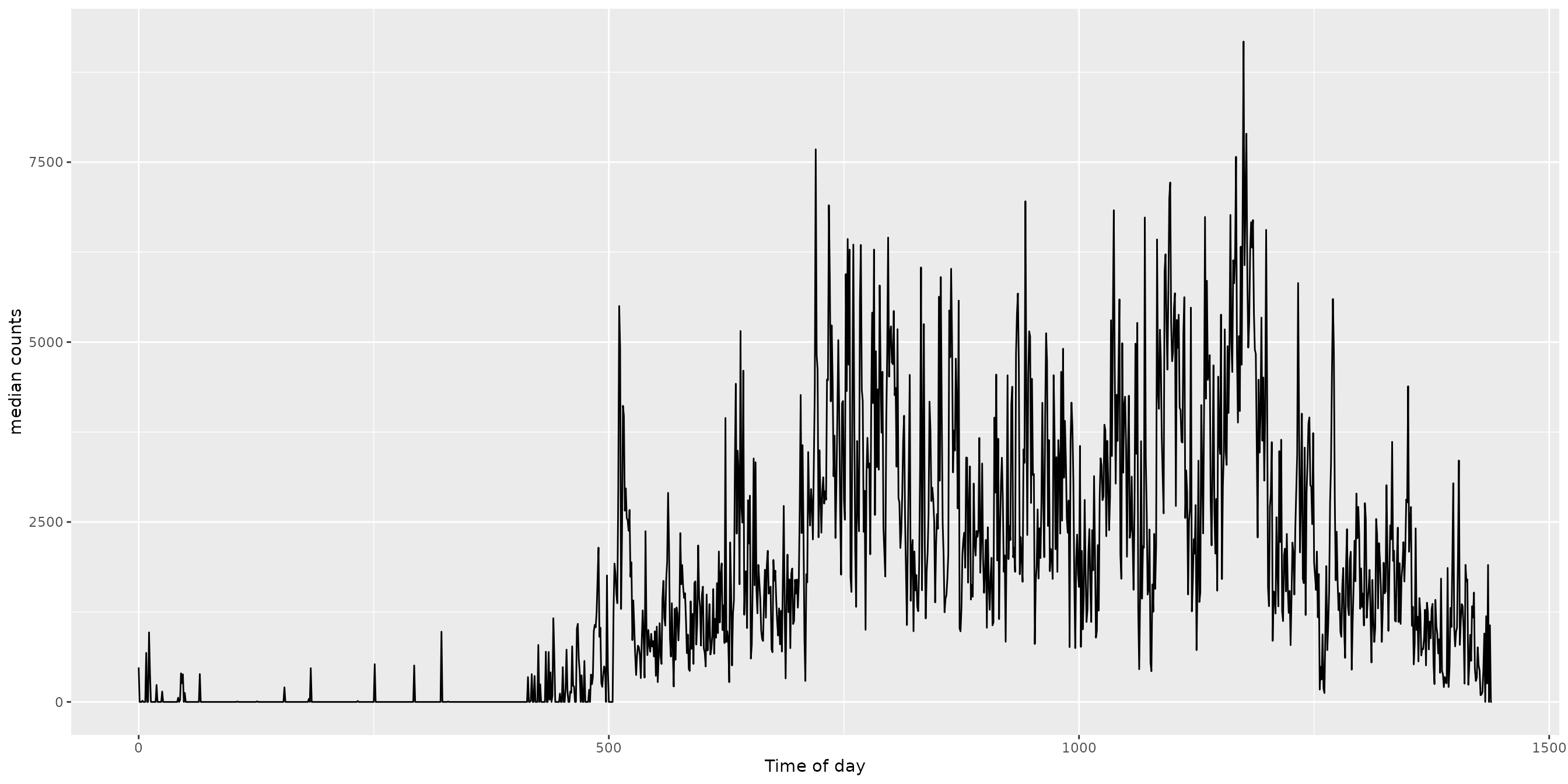

Interval annotations

Episode layers use an explicit interval table with POSIXct start and end columns. The example creates deterministic nightly windows for illustration.

sleep_windows <- data.frame(
  start = as.POSIXct(c("2017-06-03 22:00:00", "2017-06-04 22:00:00"), tz = "GMT"),
  end = as.POSIXct(c("2017-06-04 07:00:00", "2017-06-05 07:00:00"), tz = "GMT")
)

acti_plot_time(activity, counts) +
  geom_sleep_window(sleep_windows) +
  geom_day_boundary("noon", linetype = "dashed")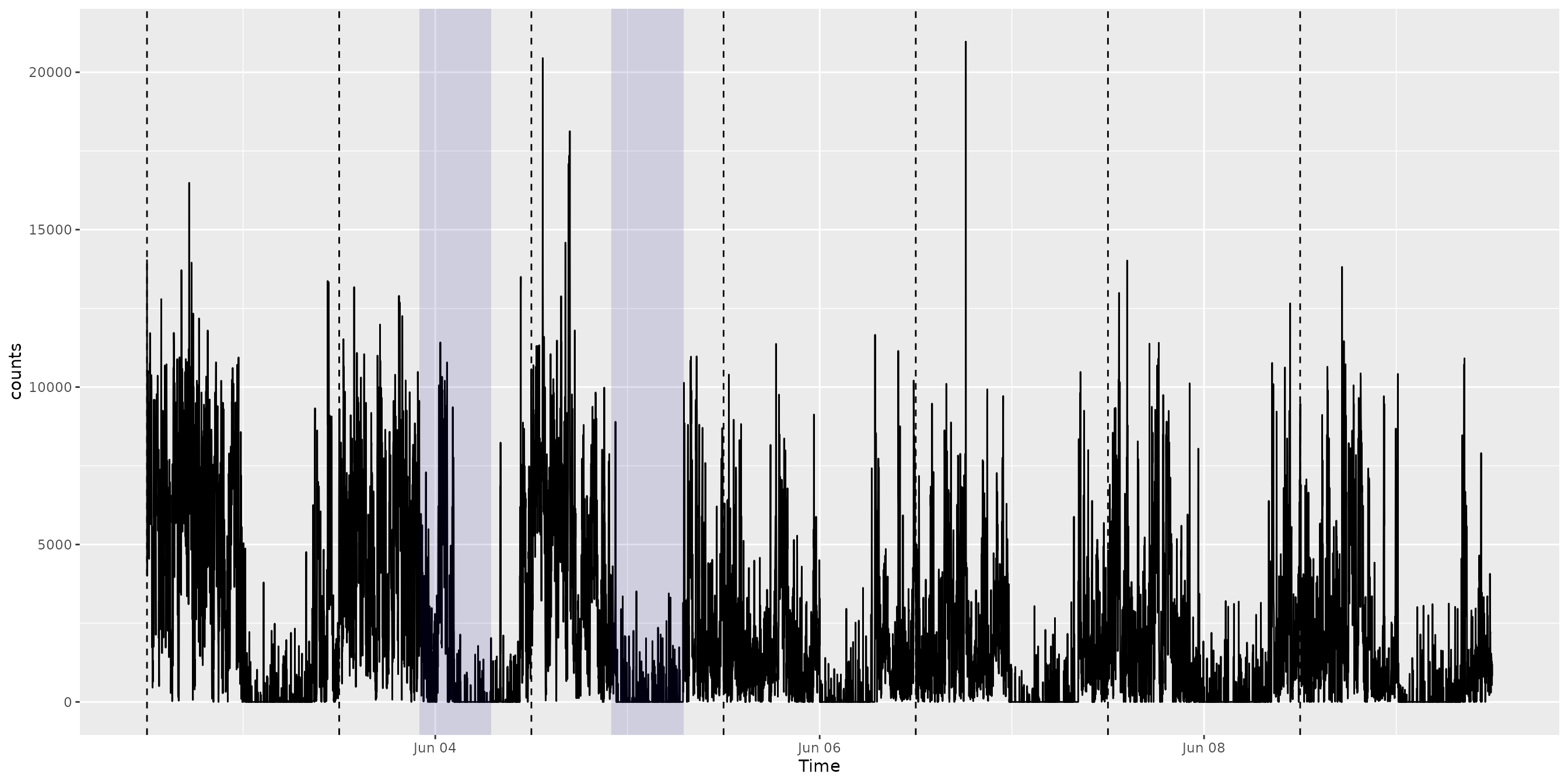

The same interval schema supports generic episodes and wear annotations.

acti_plot_time(activity, counts) +
  geom_episode(sleep_windows, fill = "grey30", alpha = 0.10) +
  geom_wear(sleep_windows)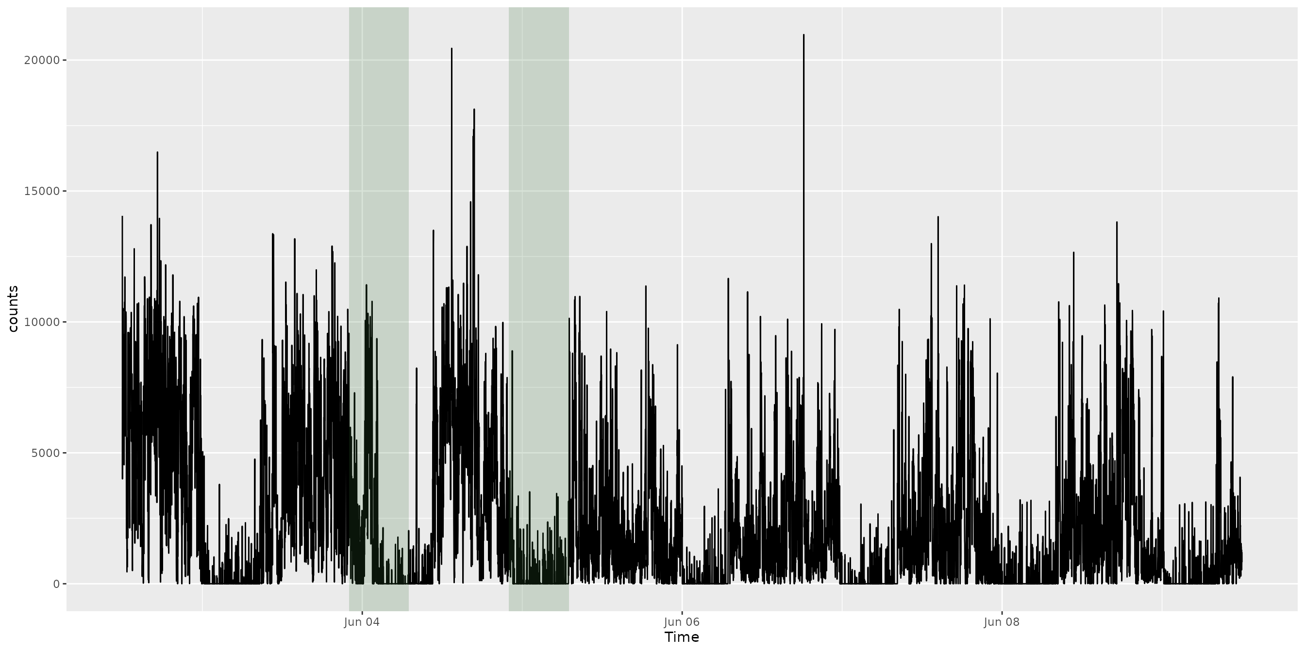

Additional lightweight annotations can mark selected activity and intensity.

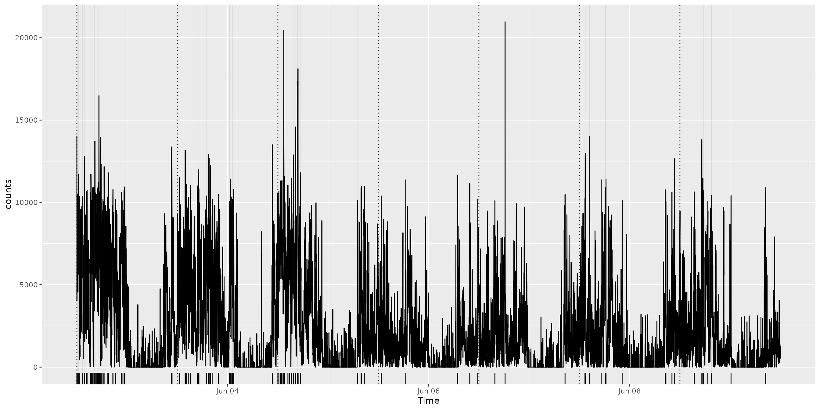
acti_plot_time(activity, counts) +
  geom_activity_rug(activity[activity$counts > 10000, ]) +
  geom_threshold_band(activity, "counts", threshold = 10000) +
  geom_time_vline(xintercept = "12:00:00", linetype = "dotted")